The Economics of Pest Management

 

The scientific study of pests and pest control strategies is often called economic entomology in recognition of the financial impact insects have on industry, agriculture, and human society in general.   To be sure, economically important insects are not always pests; we have already stressed their value as pollinators, natural enemies, producers of silk, honey, etc.   But wherever pest populations develop, their impact always results in monetary loss, either directly or indirectly.   In most cases, losses from insect pests are directly proportional to the density of the pest population — high density increases the extent or severity of damage and makes the need for control more critical.

Injury vs. Damage

Many people use the terms “damage” and “injury” interchangeably, but entomologists usually make an important distinction between them.

• Injury is defined as the physical harm or destruction to a valued commodity caused by the presence or activities of a pest (e.g., consuming leaves, tunnelling in wood, feeding on blood, etc.).
• Damage is the monetary value lost to the commodity as a result of injury by the pest (e.g., spoilage, reduction in yield, loss of quality, etc.).

Any level of pest infestation causes injury, but not all levels of injury cause damage.   Plants often tolerate small injuries with no apparent damage and sometimes even overcompensate by channelling more energy or resources into growth terminals or fruiting structures.   A low level of injury may not cause enough damage to justify the time or expense of pest control operations.   These sub-economic losses are simply part of the cost of doing business.

But at some point in the growth phase of a pest population it reaches a point where it begins to cause enough damage to justify the time and expense of control measures.   But how does one know when this point is reached?   (How many boll weevils, for example, does it take to make a cotton farmer hook up his sprayer?)   To a great extent, the answer depends on two fundamental pieces of economic information:

A.   How much financial loss is the pest causing?   and
B.   How much will it cost to control the pest?

A pest outbreak, by definition, occurs whenever the value of “A” is greater than the value of “B”.   Actual losses are relatively easy to measure in agricultural or industrial settings because commodity values are well established by commerce and trade.   But losses from household insects, vectors of human disease, and nuisance pests can be much harder to quantify.   In these cases, estimates of damage are often based on potential loss (from disease, contamination, etc.) rather than on actual or expected loss.

Economic Injury Level

The break-even point, where “A”=”B”, is known as the economic injury level.   This is the population density at which the cost to control the pest equals the amount of damage it inflicts (actual or potential).   Below the economic injury level, it is not cost-effective to control the pest population because the cost of treatment (labor plus materials) would exceed the amount of damage.   Above the economic injury level, however, the cost of control is compensated by an equal or greater reduction in damage by the pest.

The economic injury level (EIL) is often expressed mathematically by the formula:

where:

• “C”   is the unit cost of controlling the pest    (e.g., $20/acre)
• “N”   is the number of pests injuring the commodity unit    (e.g., 800/acre)
• “V”   is the unit value of the commodity    (e.g., $500/acre)
•  “I”   is the percentage of the commodity unit injured    (e.g., 10% loss)

For the example given above, the economic injury level would equal 320 insects per acre:

The economic injury level is usually expressed as a number of insects per unit area or per sampling unit.   Occasionally, when the insects themselves are difficult to count or detect, the economic threshold may be based on a measurement of injury (e.g., leaf area consumed or number of dead plants).

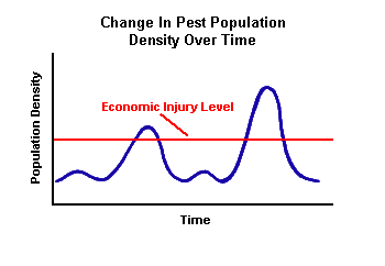
It is important to recognize that the economic injury level is a function of both the cost of pest control and the value of a commodity or product.   Some commodities may be worth so little that it is never worth saving them from insect injury.

More about
Different Values The value of other commodities may be so great that any level of infestation is worthy of control.  Because of its dependence on both cost and value, the economic injury level can be calculated only after establishing a value for the damaged commodity or product.  In practice, this can sometimes be a difficult task because different people have different values.

Economic Thresholds

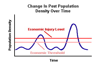
The economic injury level is a useful concept because it quantifies the cost/benefit ratio that underlies all pest control decisions.   In practice, however, it is not always necessary or desirable to wait until a population reaches the economic injury level before initiating control operations. Once it is determined that a population will reach outbreak status, prompt action can maximize the return on a control investment.   Since there is usually a lag time between the implementation of a control strategy and its effect on the pest population, it is always desirable to begin control operations before the pest actually reaches the economic injury level.

Consequently, entomologists define a point below the economic injury level at which a decision is made to treat or not treat.   This decision point is called the economic threshold, or sometimes the action threshold.   It is the decision point for action — the pest density at which steps are first taken to ensure that a potential pest population never exceeds its economic injury level.   The economic threshold, like the economic injury level, is usually expressed in units of insect density or in terms of an injury measurement.   The economic threshold is always lower than the economic injury level in order to allow for sufficient time to enact control measures.

Surveillance of Pest Populations

Effective use of economic thresholds in the management of insect populations depends on accurate measurements of population density as well as reliable predictions of population growth trends.   Since it is not practical to count all the flies in the barnyard or all the boll weevils in the cotton field, entomologists depend on sampling strategies to estimate density and distribution.   Hundreds of sampling methods have been devised and entomologists continue to develop and refine their techniques.

An “ideal” sampling strategy requires minimal effort and gives an accurate and reproducible measure of the density and/or distribution of an insect population.   In practice, such “ideal” methods do not exist.   Every technique is inherently biased in some way.   One method may be better than another for a particular pest or situation, but no sampling process is totally random, objective, and repeatable.   The most widely used techniques, such as sweep nets or bait traps, do not measure absolute density of pest populations, they are only relative measures (yardsticks, in a sense) that may be used as estimates of population density once they are properly “calibrated” through experimentation and comparison with other sampling techniques.

Sex pheromone traps, for example, may attract male peachtree borers from several miles downwind.   Without compensating for such immigration, trap catch data would greatly exaggerate the size of a local moth population.   Similarly, sweepnet samples of alfalfa weevils tend to underestimate the numbers of small larvae in a field (relative to adults and large larvae) because early instars hide within the plant’s terminal growth and are not easily knocked out during sweeping.

Analysis of Sampling Data

Simple, descriptive statistics are essential for interpreting data collected in any replicated sampling scheme.   Regardless of how data is gathered, whether as continuous measurements (e.g., leaf area consumed), in the form of numerical counts (e.g., number of beetles per plant), as ordinal ratings (e.g., on a scale from 1 to 10), or in binomial form (e.g., presence/absence), there is always some degree of uncertainty about its accuracy.   Statisticians call this uncertainty “variance”.   It arises both from experimental error (inability to precisely replicate all conditions in each sample) and from the natural variability that is a characteristic of all biological systems (e.g., the number of leafhoppers collected in 25 sweeps at dawn may be quite different from a similar sample taken that evening in the same field).   Good sampling strategies are designed to minimize variance in order to give the most reasonable “estimate” of population size.

The mean, variance, and standard error are the calculations most commonly used to evaluate sampling results.  The mean is simply an arithmetic average of data values.  It is one of several ways to describe a range of numbers.  The variance (sum of squared deviations from the mean divided by number of observations), and the standard error (square root of the variance divided by the mean) are measures of how far the other data values tend to stray from the mean.

Statistical tools provide a way to find and measure the variance in many different types of data.   Columns A and B (below) have the same “average” values (50), but the variance of column A is obviously much lower than column B.   If these numbers represent sample data collected from a single population, an estimate of population size based on the numbers in column B would be regarded with a great deal more skepticism than a similar estimate based on the numbers in column A.   In general, larger numbers of samples provide more trustworthy estimates of population density.

Column A	Column B
51 49 51 48 50 49 52	12 79 23 67 31 47 91

By knowing the amount of variance in sample data, it is possible to calculate a range of values, a confidence interval, that includes the upper and lower boundaries of our faith in the reliability of the samples.   A 99% confidence interval means that the probability of data falling outside a given range of values is only 1 in 100.   Confidence intervals can be set at any level of certainty, but in practice, most pest management decisions are based on 95-99% confidence levels.   A lower confidence level is associated with an increased risk of uncertainty in the development or outcome of a pest outbreak.   The farmer’s decision to treat or not treat a pest population has to be made with as little risk as possible.   If the pest population is larger than indicated by sample data, failure to treat could result in total destruction of a crop.   On the other hand, if the population is smaller than indicated by sample data, money would be wasted by a decision to treat.

Sequential Sampling

Although it is fairly easy to sample for some insects, many pest management systems utilize sampling protocols that are fairly time consuming and labor intensive.   Whenever large numbers of samples are needed to achieve an adequate level of confidence, it may be possible to use a sequential sampling system that saves time and effort by concentrating mostly on populations that are closest to the economic threshold.   Sequential sampling systems are relatively new in pest management, but they are based on well-established rules for determining confidence intervals for sample data.

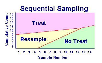
Unlike regular sampling protocols that require a fixed number of replications (usually 10-100), sequential sampling systems are designed to evaluate the data at the end of each sampling step.   The total number of samples is variable, depending upon whether the cumulative data falls inside or outside of predetermined confidence intervals.   Relatively few samples would be needed to recognize that a population is very small (well below the economic threshold) or very large (well above the economic threshold).   But a larger number of samples (higher confidence) would be needed to decide whether an intermediate population should be treated or not treated.

In most sequential sampling systems, there are three different outcomes possible at the end of each sampling step:

1. If the cumulative total of pests exceeds an upper threshold value, then conclude that the population is large enough to warrant control actions.   Stop sampling and prepare to enact control measures.
2. If the cumulative total of pests is beneath a lower threshold value, then conclude that the population is small and warrants no control actions.   Stop sampling (at least for awhile) and leave the population untreated.
3. If the cumulative total of pests is between the upper and lower threshold values, then no conclusion is possible yet.   Sampling should continue until cumulative values reach the upper or lower threshold.